Antimony electrode
From standard electrode potential literature, we have the following information:
(A) With reference to standard hydrogen electrode (E∅ = 0.000 V)
Medium | Reduction half equation | Ef/V |
Alkaline | SbO2- (aq) + 2H2O(aq) + 3e- | -0.639 |
Neutral or slightly acidic | Sb2O3(s) + 6H+(aq) + 6e- | +0.150 |
Acidic | SbO+ (aq) + 2H+(aq) + 3e- | +0.204 |
Clearly, according to the Nernst equation, half-cell formed by oxidation state (III) species SbO2-, Sb2O3 and SbO+ involves H+ or OH- and generates e.m.f. which depends on concentration of H+(aq) over the entire pH range.
Usually, commercial reference electrode for full cell pH measurement is the Ag/Ag+(aq.) (in gel buffer) reference electrode. For the suggested experiments in Program (2), we use the less expensive alternative which is a low-cost Cu/Cu2+(aq) half-cell.
(B) With reference to standard copper/copper (II) ion electrode (E∅ = +0.340 V)
Medium | E∅/V, w.r.t. standard hydrogen electrode | E∅/V, w.r.t. standard Cu/Cu2+ |
Alkaline | -0.639 | – (+0.340 + 0.639) = – 0.979 |
Neutral or slightly acidic | +0.150 | – (+0.340 – 0.150) = – 0.190 |
Acidic | +0.204 | – (+0.340 – 0.204) = – 0.136 |
Primary cell formed by antimony pH measurement:
– +
Sb(s) | Sb(III) | H+ (aq) || Cu2+ (1M) | Cu(s)
Theoretically speaking, a chemical cell formed by Sb/Sb(III) half-cell and a Cu/Cu(II) reference half-cell will generate a potential difference covering the most commonly encountered pH range of 1 to 13, from 0.136 V to 0.979 V, with antimony as the negative pole and copper as the positive pole.
Mainly due to input resistance cannot meet the demand of an order of 1000 MW, e.m.f.s. measured by a commercial DMM do not agree with the theoretical expectation, but are still very close, as shown by the following graph:(A
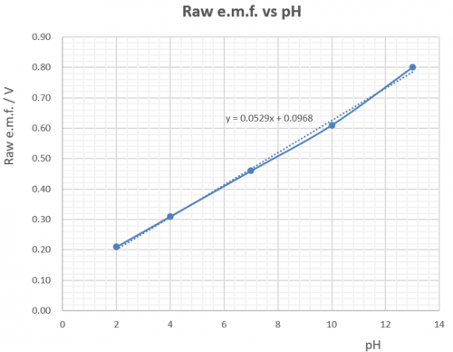
(Fig. 119) Primary cell e.m.f. measured by a DMM vs pH
The good thing about the findings is that (i) a linear relationship between e.m.f. and pH is observed, (ii) internal resistance of the cell formed is low which favours easy e.m.f. measurement by a low cost DMM and (iii) e.m.f. output is stable.
Glass electrode
Primary cell formed by glass electrode pH measurement:
+ –
Ag(s) | AgCl(s) | H+ (aq) || glass membrane | buffer solution | Pt(s)
For glass electrode, as revealed by most literature, a true linear relationship is found between e.m.f. and pH over practically the entire pH range, notably from pH 0 to 12 (except the acidic and alkaline error ranges at the two extremes). Also, glass is resistant to corrosion by most chemicals. However, as minute current is allowed to pass through glass membrane, cell formed by glass membrane electrode has extremely high internal resistance (in the order of 1010 W). Although nowadays chips for electronic circuits are capable of handling very high input impedance, this still causes problem in obtaining stable and reproducible readings, as the instrument is vulnerable to “noise” interference.
Summary
Antimony electrode | Glass electrode | ||
| * | Almost linear relationship between cell emf and pH, from pH 2 to 12 | * | True linear relationship between cell emf and pH, from pH 0 to 12, except the acidic and the alkaline error ranges |
| * | Low cell internal resistance. Conventional plug and socket input will suffice. | * | Extremely high cell internal resistance. BNC plug and socket input are required |
| * | Slower response, less sensitive to low pH ranges | * | Faster response, sensitive to all regions of the linear pH range. |
* | Readings reproducible and stable |
* | Today’s high-tech high impedance input fabrication enables reproducible and stable readings, but still liable to external interference |
| * | Measurement principle explained at school level | * | Advanced measurement principle |
| * | Sturdy | * | Fragile |
| * | Lifetime dependent on mass of electrode | * | Limited glass membrane life time |
| * | Liable to chemical corrosion | * | Resistant to chemical corrosion |
| * | Easy fabrication | * | High-tech fabrication needed |
| * | Low-cost | * | Expensive |
Examination of the advantages and disadvantages between antimony and glass electrodes reveals that antimony electrode is a better choice than glass electrode for school use.
Innovative “Salt-plug”
A small piece of freshly prepared filter paper strip wetted with sat. KNO3 solution is usually employed as a salt bridge for school use. In the experiment, an alternative way is used which involves a small section of wooden toothpick soaked with sat. KNO3 solution and let dried. A number of such small pieces of home-made instrument are readily available as innovative “salt-plugs”. Using them is very simple: First fill the reference electrode glass tubing chamber with 1M CuSO4 solution, and then insert the “salt-plug” into the opening of the glass tubing chamber. Air bubbles in the chamber are not allowed as they may cause the copper metal and the copper (II) sulphate solution out of contact (Fig. 120, 121, 122 and 123). Lower the finished reference electrode, together with the antimony electrode, into the testing solution for pH measurement.
“Salt-bridges” need to be freshly prepared for each measurement. However, “salt-plugs”, after rinsing, can be used repeatedly until the end of the experiment.
 |  |  |  |
(Fig. 120) Use a micro-tip plastic pipette to fill the small chamber with 1M CuSO4 solution | (Fig. 121) Solution should be filled to the top of the small tubing. Slight excess as judged by an almost overflow. | (Fig. 122) Insert the “salt plug” | (Fig. 123) Prepared copper /copper sulphate electrode with no air bubbles |
Two modes of practical pH measurement by antimony electrode
Direct-reading mode
Theory of measurement
As its name implies, direct reading mode refers to the instrument displays a value of 40 for a solution of pH 4.0, a value of 70 for pH 7.0 and so on.
The constructed probe immersed in aqueous solution forms a primary cell: Sb(s) | Sb (III) | H+ (aq) || Cu2+ (1M) | Cu(s), the cell output e.m.f. varies linearly with change of pH value. If it is fed directly to a DMM, a graph looking like Fig. 119 will be obtained. Unfortunately, it is not a direct-reading mode scenario.
To meet the demand of direct-reading mode, the probe has to be fed to a sensor first before connecting to the DMM (Fig. 124). Upon connection, the DMM’s measuring range is selected to DC 2000 mV FSD. When the probe is immersed in an aqueous solution of pH = 4.0, the DMM will display 40 mV which is taken as 4.0. If a sample solution of pH 7.0 is used, the DMM will display 70 mV and so on. Thus, voltages can be interpreted as pH readings without reading unit. This technique is the “DMM Display Technique”. Principle behind is not new, but the usage is innovative.
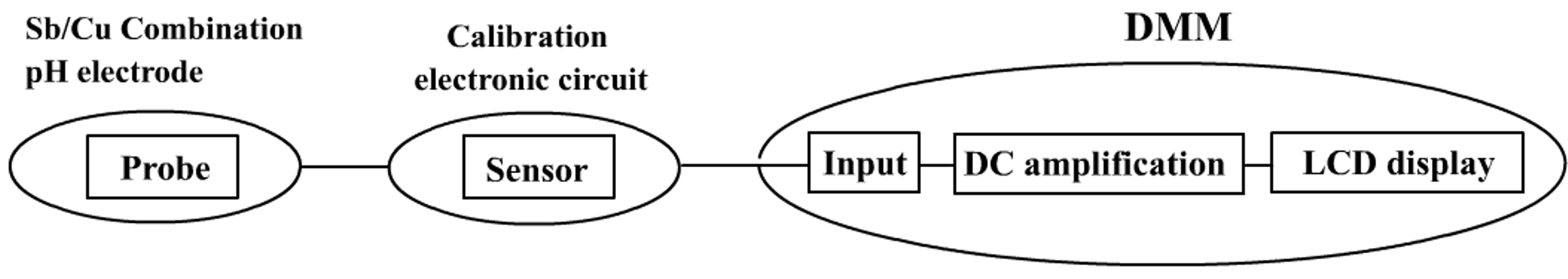
(Fig. 124) Schematic diagram of “Direct-reading mode” of pH measurement
Accuracy and sensitivity of the antimony pH electrode as designed are not decently high, but is very suitable for school use. Due to this built-in imperfection, a display accuracy of one decimal place is just good. In other words, a result of pH = 7.26 is not practical and a value of 7.3 is more realistic. To overcome this problem, there is a need to install an attenuating device and the sensor circuit as illustrated in Fig. 126 will include this part.
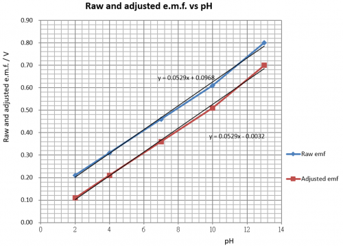
(Fig. 125) Raw and adjusted e.m.f. vs pH
pH | Adjusted e.m.f./V | “One-point” calibration | Amplification ratio | Amplified voltage/V | Attenuated (output) voltage/mV | Interpreted pH |
2 | 0.11 | — | — | (0.11 x 1.94) = 0.21 | 21 | 2.1 |
| 4 | 0.21 | — | — | (0.21 x 1.94) = 0.41 | 41 | 4.1 |
7 | 0.36 | 0.70 V | 0.70/0.36 = 1.94 | (0.36 x 1.94) = 0.70 | 70 | 7.0 |
| 10 | 0.51 | — | — | (0.51 x 1.94)= 0.99 | 99 | 9.9 |
13 | 0.70 | — | — | (0.70 x 1.94) = 1.36 | 136 | 13.6 |
Buffer solutions of pH 2, 4, 7, 10 and 13 are used for calibration. A 0.100 M NaOH solution can be regarded as a pH 13 buffer solution.
(Fig. 126) “One-point” calibration with amplified voltage plotted against pH
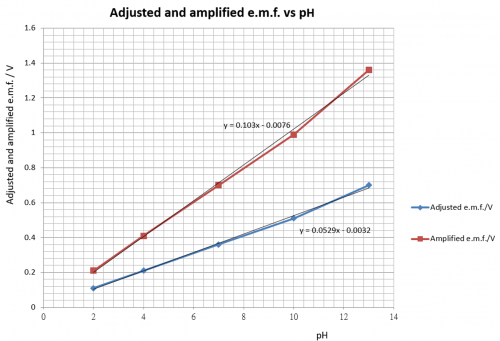
Because only one pH value, i.e. pH 7 is selected for calibration, this method is called “one-point” calibration. After adjusting the raw e.m.f. and followed by a 1.94 amplification factor, a relationship of 100 mV per pH will result. That is to say, pH = 7.00 is displayed as 700 mV, pH = 4.47 is displayed as 447 mV etc. As mentioned earlier, pH value registered by antimony pH electrode is only good for one decimal place accuracy, there is a need to attenuate the output voltage by a factor of 1/10. Thus, instead of 100 mV per pH, the final voltage output bears a relationship of 10 mV per pH, or pH 7.00 is displayed as 70 mV and pH 4.47 is displayed as 45 mV and so on.
Sensor circuit and description
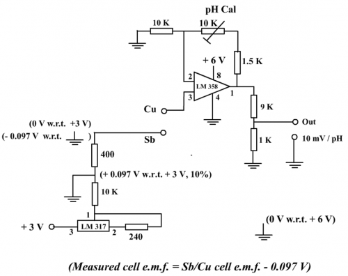
(Fig. 127) Sensor circuit
(i) Power supply
The sensor circuit employs two power supplies. One (3V) for the adjustable voltage regulator LM 317 to generate a negative voltage reference, and the other (6V) for the Vcc of Op Amp LM 358. They are readily supplied by using three button-type 3V lithium batteries, two of which are connected in series to obtain 6V (Fig. 132). Adjustable voltage regulator LM 317 is used because the chip can handle low input voltages (i.e. 3V). Linear dual Op Amp LM 358 is chosen for the amplification stage because this IC needs only single power supply (i.e. it does not need a negative power supply).
(ii) Negative voltage reference
Adjustable voltage regulator LM 317 is connected by peripheral resistors to output a regulated voltage. The 400 W resistor (or suitable adjustment) taps a reference voltage of + 0.097V (Program (1), page 102). This positive voltage reference source is then connected to the ground of the power supply (6V) of Op Amp LM 358. In this way, the separate ground terminal (3V) which generates the reference voltage becomes – 0.097V. By applying this negative voltage, raw e.m.f.s are “set” and “corrected” for direct proportionality. LM 317 is not a formal voltage reference chip but it can offer a stable voltage output over a period of time. Availability and low cost are the reasons for adopting it.
(iii) Adjusting raw e.m.f.
As shown by Figure 119, graph of untreated raw e.m.f. vs pH did not pass through the origin (0 0) and resulted in an intercept of 0.097 V on the OY axis. Connecting pin 3 of LM 358 (non-inverting input) to the positive pole (Cu) of the Sb/Cu chemical cell and the negative pole (Sb) to the – 0.097V reference voltage source (Fig. 127) results in summing the two voltages, i.e Ecell and – 0.097V and the effective e.m.f. of the Sb/Cu chemical cell becomes (Ecell – 0.097) V. Theoretically, the effective e.m.f. straight line graph should pass the origin (Fig. 128).
(Fig. 128) Raw e.m.f. and adjusted e.m.f. vs pH
(Fig. 129) Adjusted and “one-point” calibrated e.m.f. vs pH
(v) Follow-up of amplification Accuracy of antimony electrode in pH measurement is not high and it is realistic to limit the numerical digital display accurate to one decimal place. For example, display 7.4 instead of 7.38 and so on. This can be achieved by installing an attenuating resistor ladder (9: 1) at pin 1 (output) of LM 358 such that the millivolt range output of 70 mV is registered instead of 700 mV. Without the attenuating resistor ladder, the output voltage is displayed as 700 mV. The circuit design itself does not warrant an accurate interpretation of, say, 7.00, e.g. two decimal places accuracy. Hence there is a need to limit the overall output to display 10 mV per pH, not 100 mV per pH. (v) Calibration summary First set the DMM to the DC 2000 mV full-scale range. Second carry out the “one-point” calibration by selecting a suitable buffer solution, say a pH 7 buffer. Place the Sb/Cu combination electrode into the buffer, connect it to the sensor which in turn is linked to the DMM. Carefully rotate the pH cal knob (10 KW variable resistor) until a steady display of 70 mV appears. “One-point” calibration is achieved and the position of the knob is kept fixed (Fig. 130). The set is ready for pH measurement. For example, if the calibrated combination electrode is placed in a solution of unknown pH and the DMM shows 55 mV, then the solution is taken as having a pH value of 5.5, and so on. All in all, criterion for the design of the sensor is: to achieve an output of 0 mV for 0 pH followed by consecutive increase of 10 mV per pH.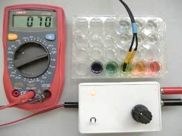
(Fig. 130) “One-point” pH 7 calibration
(v) Sensor construction
The most important objective of homemade instrument construction should be aimed at purchasing all materials from local resources. Various manipulative and electronic skills of Program (1) are assumed. Locations for electronic component and material purchase are listed in Topic 15 of Program (1). Prices of electronic components do not go up with inflation rate, instead they behave just the opposite, notably in Hong Kong. All materials, including the DMM, do not cost much.
As the whole circuit draws little current, the power source is supplied by 3 button type lithium dry cells (CR 2032), each offering a voltage of 3V. A special holder for such dry cells is used and three such holders are held together by an acrylic strip with the help of a few drops of trichloromethane (Fig. 132). Two of them (6V) are used for the power supply of LM 358 while the single one is for generating the negative voltage of – 0.097V.
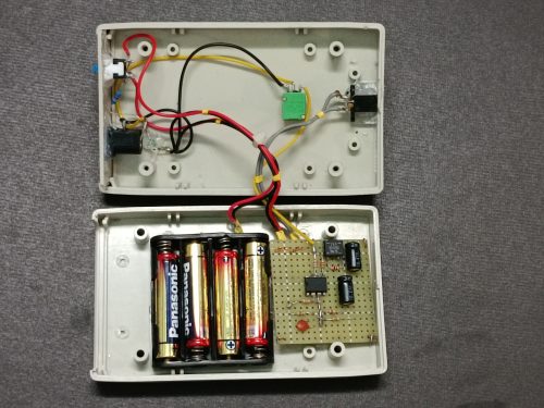
Using available electronic components, circuit as shown in Fig. 127 can be soldered onto a small universl circuit board (Fig. 131). The fabricated body can be housed in a plastic utility box measuring 10 cm x 6 cm x 2.5 cm (Fig. 132 and 133). As the box is pretty small, connecting wires and soldered components will pack together without any fixture. Upon closing the lid, a sturdy instrument will be in your hand (Fig. 133).
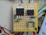 | 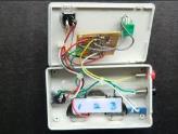 | 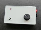 |
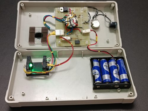
| (Fig. 131) Electronic components soldered onto a universal circuit board | (Fig. 132) Exposed interior of utility box (three 3V lithium button-type batteries are labeled as 1, 2 and 3) | (Fig. 133) Finished utility box with all components installed |
Fabrication of antimony electrode and copper/copper sulphate reference electrode
(1) Antimony electrode
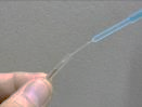
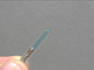
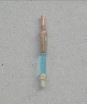
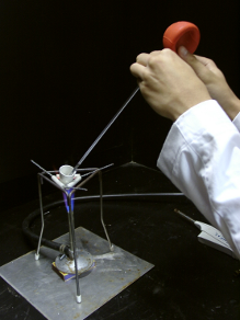
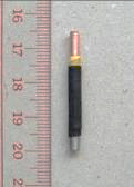
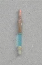
Antimony metal of A.R. grade was strongly heated in a crucible (inside a fume cupboard) until it melted (Fig. 134). The molten metal was withdrawn upward, with the help of a pipette filler or syringe into a small glass tube. The hot liquid antimony solidified inside the glass tube and the solid metallic rod was taken out by breaking the glass tubing. The prepared antimony rod is brittle and can be easily broken into small sections. Take one of the bits and solder it onto a length of copper lead for electrical conduction (antimony picks up solder easily). The metal/copper rod combination was sealed by a section of heat-shrinkable plastic tubing to form a formal pH electrode (Fig. 135) |
(2) Copper/copper(II) sulphate reference electrode and innovative “salt-plug”
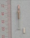
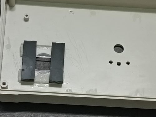
The copper/copper(II) sulphate reference electrode was constructed by using a short section of copper lead and glass tube. The copper lead was sealed to one end of the glass tube with epoxy glue, leaving a protruded thick copper wire for electrical conduction and the rest forming a small chamber for filling copper(II) sulphate solution (Fig. 136). A small “salt-plug”, constructed by using a toothpick bit, replaces a conventional filter paper salt bridge. A “salt- plug” is simply a small section of wooden toothpick soaked in sat. KNO3 solution and allowed to dry. Air bubbles are not allowed in the chamber, otherwise solution conductance will become unstable (Fig. 137) |
(3) Completed combination electrodes
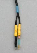
(Fig. 138) Finished Sb and Cu/CuSO4 electrode
Inspection of the above photos reveal with no difficulty in explaining the working principle of measurement based on primary cell formation. The combination electrode fits a 24 well plate nicely for experimentation.
Expt (17): Antimony combination electrode for pH measurement using sensor and “One-point calibration” (page 134)
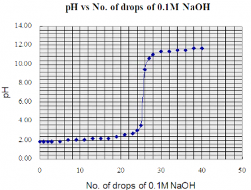
Expt (18): 0.1M HCl vs 0.1M NaOH (strong acid vs strong base) titration curve (page 136)
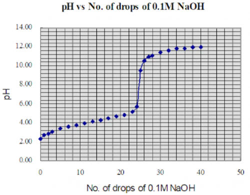
Expt (19): 0.1M CH3COOH vs 0.1M NaOH titration curve (page 139)
a. Basic Mode
Theory and method of measurement
Apart from using a sensor to carry out the direct-reading mode of measurement, a basic mode of measuring without a sensor is simpler and attains even better experimental results. It requires only the combination electrode to be directly fed to a DMM. Another way of calibration is needed for this mode.
First establish a calibration graph involving buffer solutions of pH 2, 4, 7, 10 and 13 (Fig. 139).
(Fig. 139) Graph of raw e.m.f. vs pH
Extend the almost straight-line graph (Fig. 139) so that it covers the entire pH range of 0 to 14. If a raw e.m.f. of 0.14 V is measured, then a value of pH =1.00 can be deduced from the extended graph, and so on.
With the help of a suitable spreadsheet software, e.g. MicroSoft Exel, establish a calibration regression line. Input a raw p.d. of 0.14 V will receive an immediate result of pH 1.00.
Expt (20): Basic method of antimony combination electrode for pH measurement without using sensor (page 142)
5.2 “Micro-scale Conductance Meter” and suggested Experiment (21) and (22)
Junior and senior chemistry syllabuses all include the topic of electrical conductivity of aqueous solution e.g. electrolysis or conductometric titration. One point to note: decomposition of electrolyte (i.e. electrolysis) occurs if DC current is used. Hence, measurement of conductance of aqueous solution has to use AC or oscillating current.
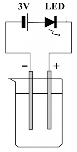
(Fig. 140) A simple LED conductance device
A lot of schools use the above device (Fig. 140) to test the strength of solution conductivity by observing the degree of brightness of the LED. It is indeed a useful and simple apparatus suitable for junior scientific activity. However, DSE Chemistry not only requires student to qualitatively differentiate solution conductivity but also to take quantitative readings. Obviously, the above device is not suitable for DSE Chemistry, let alone the associated phenomenon of electrolysis.
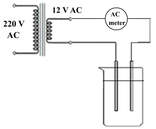
(Fig. 141) A simple low AC voltage conductivity meter
No electrolysis will occur if the city’s AC power supply is converted by a transformer to low AC voltage and this is exactly what the design shown in Fig. 141 will do. The method is traditional, not innovative or convenient. Today’s school science labs are equipped with bench low DC voltage sources which are not suitable for conductivity experiments. Installing external transformers are also clumsy.
Features of the designed micro-scale conductance meter
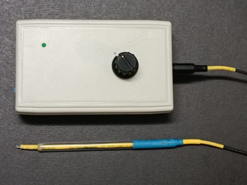
(Fig. 142) Micro-scale conductance meter
- The design employs the “DMM Display Technique” in which a commercial low-cost digital multimeter (DMM) acts as the terminal display. Instruments employing the “DMM Display Technique” is very suitable for school level quantitative measurement of reaction variables such as pH, solution conductivity or colour intensity of aqueous solutions. Principle of measurement is based on probes for these reactions output electrical signals, which after suitable amplification, can be nicely handled in the DC millivolt range measurement by all kinds of low cost DMM which provide at least an input resistance of 10 MW, ensuring only slight loss of source signal.
- Commercial conductivity meters commonly use “mS/cm” as reading unit. Meaning of the unit is usually not taught in school-level lessons. The design aims at doing away with such kind of reading units. When the conductivity probe is connected to the sensor which in turn connected to a DMM set at the DC 2000 mV range, and by short circuiting the two electrodes of the probe, the sensor outputs a pre-set maximum voltage of 100 mV and this value is treated as full conductance (i.e. 100). If a value of 34 mV is displayed when an unknown solution is tested, the electrical conductivity of this solution is taken as having 34/100 strength of full conductance (Fig. 143). This offers a “user-friendly” and less threatening situation for dexterity less competent school students.
- Circuit design gives an output voltage around 500 mV which can be attenuated to 385 mV (for details please go over page 63) and this means we can set the full scale 300 V to a higher voltage, say 300 mV, or a full scale of 300 instead of 100. The advantage of using this method is that one more digit of voltage can be displayed. For instance, using this way of calibration set at 300, a display of 123 can be achieved compared with a value of 41 employing the full-scale calibration set at 100 under the same condition. In other words, this method increases the accuracy of measurement.
- The design uses an Op-Amp relaxation oscillator to generate a single frequency alternating square wave signal source for electrical conductivity (Fig. 152). This way avoids electrolysis of the testing solution, as shown in Figure 164.
- The sensor employs a voltage follower circuit for a unity gain output with no voltage inversion (Program (1) Topic 8.3.1, page 80). This kind of buffered circuit is ideal for obtaining a stable, interference (noise) free and very low drift output voltage.
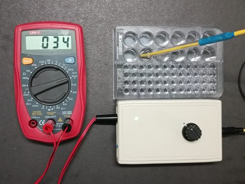
(Fig.143) Micro-scale conductance meter in operation involving the miniature probe, sensor, DMM and a 24-well plate
Instrument Construction
(1) The conductivity probe
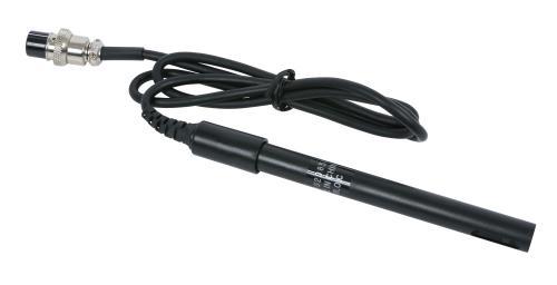
(Fig. 144) A commercial conductivity probe
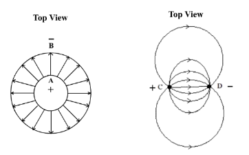
Professional conductivity probes (Fig. 144) commonly use concentric cylindrical plates A and B as electrodes, because the electric field established between the plates is evenly distributed and varies linearly with the applied ac potentials (Fig. 145). Upon calibration, concentration of a testing solution can be calculated mathematically by conductivity measurement (limited by a range of low concentration and at a fixed temperature, actual mathematical relationship involving all kinds of mobile ions of opposite charges is quite advanced, internet search). Commercial conductivity meter incorporates built-in electronic calculation mechanism and display solution conductivity finally in “mS/cm” unit. The intention of instrument construction in Program (2) is homemade, skills required for making such professional probes are not realistic for average people.
A simple design of parallel rod type conductivity probe is to make use of nichrome wire. Two sections of insulated parallel nichrome wire are used as electrodes. The electric field formed by two ends of nichrome wire C and D is curved instead of linear (Fig. 146). This is not important as long as the field is regularly distributed. If the same calibration is attempted, mathematical calculation of concentration of a sample solution is difficult. However, graphically and not mathematically, a non-linear calibration line in this case is equally good for the determination of relative concentration of sample solutions. (Note: to avoid electrolysis, AC voltage should be used instead of DC voltage, and that is exactly the main job of the sensor)
|
|
|
|
(Fig. 145) Evenly distributed electric field developed between two cylindrical electrodes A and B |
(Fig. 146) Unevenly distributed electric field developed between electrodes C and D in rod form |
Parallel rod type conductivity probe is not difficult to be made. A miniature design using nichrome wire that can fit wells of a 96 well-plate can be constructed as follows:
(a) Prepare two 13 cm long nichrome wire (with suitable stiffness) as conductivity electrodes. Nichrome wire is used because it is very resistant to air oxidation, as shown by its ability to restore to its initial cool state immedciately after becoming red hot on passing current. It is also inert to water corrosion.
(b) Seal one of the wires by heat-shrinkable plastic tubing, exposing part of the two ends for electrical conduction.
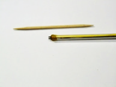
(c) Leaving the other wire remaining untreated, insert at the same time both wires into a 10 cm long glass tubing with a diameter just fit both of them. The two protruded parts are for electrical conduction. Seal one end of the glass tubing with epoxy glue. This part acts as the head of the probe (Fig. 147). The other end is partly covered by a section acrylic tubing, the main purpose is to make the glass tubing body less vulnerable to breakage and also make the probe looks more professional.
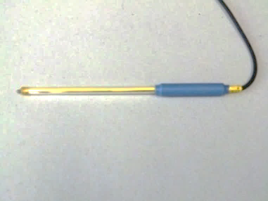
(d) The acrylic tubing end encloses a cable for signal output. Nichrome wire does not pick up solder and the joints between the nichrome wire and the copper wires inside the cable are done by tight sealing with heat-shrinkable plastic tubing (room for creative thinking). Layers of heat-shrinkable plastic tubings are used to insulate the two output lead nichrome wires. A final touch is to use heat-shrinkable plastic tubing again for a professional appearance (Fig. 148).
|
|
|
| (Fig. 147) Size of the head of the probe, compared with a tooth-pick |
(Fig. 148) Finished conductivity |
(2) The Sensor
Pre-requisite for working with the design of micro-scale conductance meter is the electronic and manipulative skills acquired in Program (1). The three main parts of the sensor are (i) an Op-Amp relaxation oscillator generating a high frequency square wave signal as ac power source, (ii) full-wave rectification of the conducted ac current and (iii) a voltage follower circuitry for stable voltage output. The whole scheme is illustrated as follows (Fig. 149).
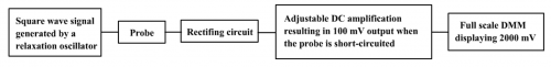
(Fig. 149) Flow chart for the design of a micro-scale conductance meter employing the “DMM DisplayTechnique”
(i) Relaxation oscillator
The important part of the sensor circuit is a signal generator. For the design, a “black-box” approach is adopted which concentrates only on the input/output requirements. We have Op-Amp IC, capacitor and resistors at our disposal and we want to generate a continuous chain of propagating AC electrical signals of frequency 5000 Hz. Revise “relaxation oscillator” of Program (1), Topic 8.3.2 (e) for the following typical relaxation oscillator circuit diagram.
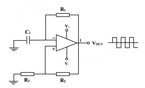
(Fig. 150) A typical relaxation oscillator circuit diagram
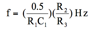
The generated frequency is represented by the following equation:
(ii) Sensor circuit diagram
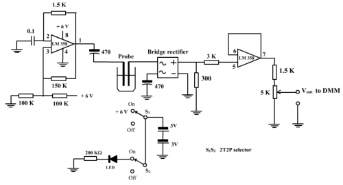
(Fig. 151) Sensor circuit of micro-scale conductance meter
(iii) Circuit description
Sensor circuit of micro-scale conductance meter (Fig. 151) can be broadly divided into 3 parts:
a. One unit of LM 358 (involving pins 1, 2 and 3) is connected as a relaxation oscillator. According to the formula of frequency generation by a relaxation oscillator:
![]()
Frequency can be calculated by suitable substituting values for C1, R1, R2 and R3. For the design, C1= 0.1mF, R1 = 1.5K, R2 = 150K and R3 = 100K, hence
![]()
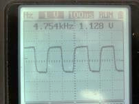
(Fig. 152) Frequency of square wave signal generated by the circuit.
Slight deviation from a theoretical value of 5 K is due to error of the component parts
b. Output ac square wave signal is allowed to pass through the mini conductivity probe and fed to a bridge rectifier for full-wave rectification, resulting in a raw dc signal with only positive cycles.
c. This voltage is fed through the 3K W resistor to a unity gain voltage follower (Program (1), page 93) formed by the other unit of dual Op-Amp LM 358 (involving pins 5, 6 and 7). The measured output voltage of 500 mV through pin 7 is attenuated by a resistor ladder consisting of a 1.5K W resistor connected in series with a 5K W variable resistor and taps 385 mV by the 5K W variable resistor (500 x mV or 385 mV). By adjusting the 5K W variable resistor, a full conductance (i.e. placing a metallic conductor between the ends of the probe) display of 100 mV, 200 mV and 300 mV can be achieved. The procedure is exactly the calibration for a FS of 100, 200 or 300. For experimentation, by setting at a FS of 100, if the sensor registered a voltage of, say, 34 mV for a testing solution, then this value represents 34/100 of the full strength of conductance, or simply 34 % strength. Alternatively, if the 5K W variable resistor is preseted to 200 mV FSD, a reading of 68 mV will result. In this way, there is no need to use unit mS/cm to indicate experimental results, thus demonstrating the usefulness of the “DMM Display Technique”.
(iv) Complete sensor construction
a. Semi-finished circuit board:
Nearly all electronic components can be soldered onto a small universal circuit board. Before the actual soldering, estimate the best position for each component to be inserted onto the board. Allow external wires for connection to components outside the board, like the 5K variable resistor, 6V battery power source, ON/OFF mini switch, panel LED and the DC jacks (Fig. 153 and 154).
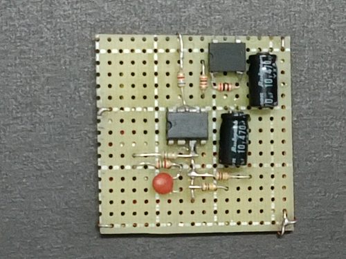 | 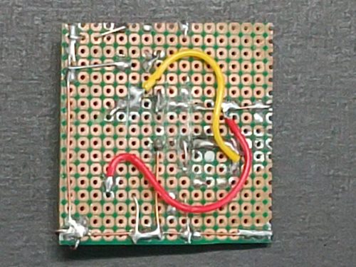 |
| (Fig. 153) Semi-finished universal board (front view) | (Fig. 154) Semi-finished universal board (back view) |
b. 6V battery power source:
A battery holder housing four 1.5 V size AAA dry cells acts as a 6V power source (Fig. 155)
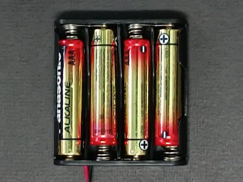 |  |  |
| (Fig. 155) 6V power supply | (Fig. 156) Utility box | (Fig. 157) Lid with noles |
c. The case:
he case of the sensor is a small plastic professional utility box measuring 120 mm (length) x 70 mm (width) x 25 mm (depth) (Fig. 156). Holes are drilled in the lid to accommodate the 5K W variable resistor, the panel LED and the probe input socket (Fig. 157). Holes of socket for the push-on/push/off mini-switch and the ouput to DMM are drilled in the side sheet of the bottom of the box (Fig. 158).
| (Fig. 158) Holes of the bottom of the box | (Fig. 159) Box with various holes |
(d) Whole assembly:
The 5K W variable resistor is fixed onto the lid, completed by capping the axle with a turning knob. The soldered pre-assembled universal circuit board is connected to various junction points of the circuit, namely the 6V holder combination, the panel LED, the 5K W variable resistor, the mini push-on/push-off switch, jacks for the probe and output to the DMM (Fig. 160). The whole assembly is kept stationary by the wires joining the circuit board (Fig. 161).
(Fig.160) Interior open view of assembly |
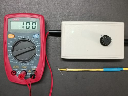
Methods of “Short-circuit” calibration
First select the DC 2000 mV range of the DMM. Connect the mini-probe to the sensor and the output plug to the DMM. Use a thread of metallic wire to short-circuit the electrodes of the probe. Alternatively, one can use a short-circuited probe plug. Carefully adjust the knob until the DMM display a value of 100 (Fig. 161,162). The position of the knob is kept fixed. Having done this, the instrument is calibrated and ready for conductivity measurement with a full-scale display of 100.
|
|
(Fig. 161) “Short-circuit” calibration method A | (Fig. 162) “Short-circuit” calibration method B |
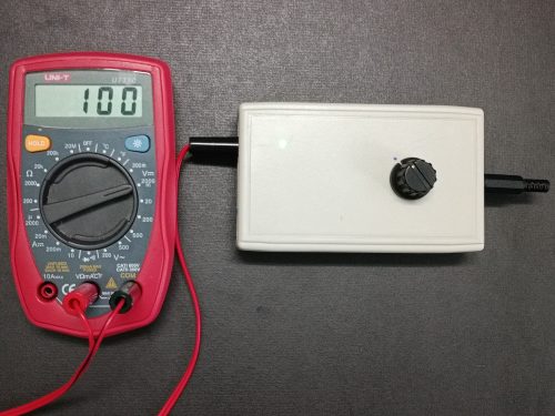
Measurement of conductivity
If the probe is placed in a sample solution and indicates a DMM value of 34, this is interpreted as the solution having a 34% conductivity compared with 100% full conductance (Fig. 163). No electrolysis is occurred while the experiment is going on (Fig. 164).
(Fig. 163) A testing solution showing 34/100 conductivity | (Fig. 164) Absence of electrolysis during conductivity measurement |
Expt (21): Micro-scale investigation of conductance of electrolytes (page 149)
Expt (22): Conductometric titration (page 157)
5.3 An affordable, sensitive, stable and user-friendly colorimeter with suggested Experiments (23), (24), (25) and (26)
Introduction
Eyes of human beings are able to differentiate relative positions of objects (sensitive to electromagnetic wave phase difference), colour detections and their relative intensities (sensitive to wavelengths and their magnitudes of amplitude). With these features, our eyes are excellent natural panchromatic and 3D colorimeters. They can tell the presence of various colours and their brightness, but are not capable of quantifying colour intensities. For instance, we may say an object is deep green, but we cannot tell the greenness is 7th or 8th degree out of a maximum of 10 (if there exists). Even so, we still use eye inspection to determine semi-quantified intensity of colour solutions with some confidence.
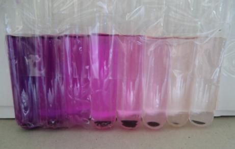
1. Concentration of a KMnO4 solution by eye inspection
| 1. | Using a pipette, transfer 10 cm3 4 x 10⁻³ M KMnO4 into test tube (1). |
| 2. | Transfer 10 cm3 of the prepared solution into another test tube, add an equal volume of deionized water, label it as test tube (2) and stir well. |
| 3. | Transfer 10 cm3 of solution of test tube (2) to another test tube, add an equal volume of deionized water, label it as test tube (3) and stir well. |
| 4. | Repeat step (3) five times, thus prepare test tubes (4, 5, 6, 7 and 8). The following table lists the result of such preparations: |
| Test tube | Conc. of KMnO4/ x 10-4mol dm-3 |
| 1 | 40.00 |
| 2 | 20.00 |
| 3 | 10.00 |
| 4 | 5.00 |
| 5 | 2.5 |
| 6 | 1.25 |
| 7 | 0.625 |
| 8 | 0.3125 |
| 5. | Arrange the 8 prepared test tubes in a roll by using a test tube rack or clear adhesive tape (Fig. 162). |
| 6. | Place a KMnO4 solution of unknown concentration (solution X) near the array. Determine which test tube of the array matches X. Concentration of X will be that of the selected test tube. |
2. Concentration determination of colour solution by a colorimeter
The above eye inspection method shows human eye is a natural colorimeter. The method is simple but is limited to only semi-quantification. However, it brings out an important step, i.e. alignment or calibration. Fig. 165 is an alignment board for matching and hence concentration determination. Although optical nerve system of the human eye is very complicated, as a kind of sensor, it can only differentiate colour variation in term of types and brightness. It lacks any kind of quantitative calibration mechanism. So, quantifying solution colour intensity needs an instrument, a colorimeter. Unlike the complicated optical nerve system of the eye, working principle of a colorimeter concentrates only on the sensor function. It uses LDR or photocell as light detector. Variation of current through the LDR due to change in monochromatic colour intensity is quantified by electronic device. Colorimeter sensor has to be calibrated before use, we cannot pick up one and start the experiment.
3. An affordable, sensitive, stable and user-friendly colorimeter
a. Features of the design
i.The designed colorimeter (Fig. 170) employs the “DMM Display Technique”. It uses low cost commercial DMM as terminal digital display for more than one kind of experiment. The innovative technique was mentioned in Topic 5.1 and 5.2. The same method is used again in the measurement of light intensity in a colorimeter. Same as the earlier two sensor designs, final output is fine tuned to display values ranging from 0 mV to 100 mV and are recorded as experimental results with numbers carrying no unit.
ii. Conventional colorimeters all use “absorbance” or “transmittance” as display units. One needs to understand Beer’s law and its associated logarithmic equation in order to use “absorbance” as a unit. Most high school chemistry syllabuses do not include such topic and teachers have to do related pre-lab discussion before the lab session involving colorimeter.
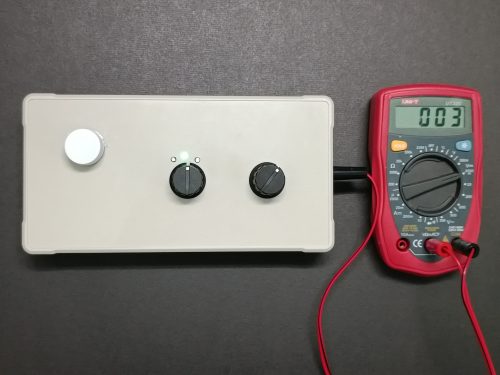
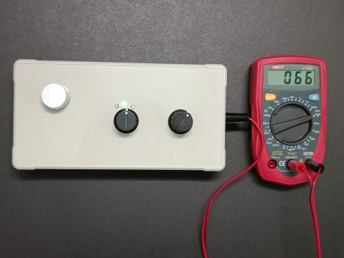
The easiest way to overcome the problem is to get rid of the measurement unit. The “DMM Display Technique” exactly fulfills the requirement. The circuit is designed to output 100 mV when a blank reference solution is irradiated with a selected monochromatic light and a 0 mV display in complete darkness (Fig. 168, 169). If a colour sample solution shows 66 mV (Fig. 167), then this solution is interpreted as having a 66% strength of transmittance using the same irradiation wavelength. In other words, the design deals with “% transmittance” only. Easy “user-friendly” handling as such is at an advantage to dexterity less competent school students.
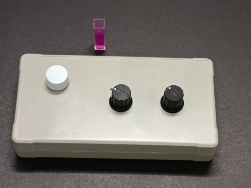
iii. Unlike school colorimeters, professional cuvette and not test tube is used (Fig. 166).
iv. School colorimeters normally use RGB filters to generate near monochromatic light source for irradiation. As blue LED became popular, tri-colour LEDs were also available in the market. These tri-colour LEDs emit near monochromatic red, green and blue light, they can replace monochromatic filters and act as light source (Fig. 167).
| (Fig. 166) Plastic cuvette and sensor | (Fig. 167) RGB tri-colour LED light source and cuvette slot | (Fig. 168) Blank sample transmittance |
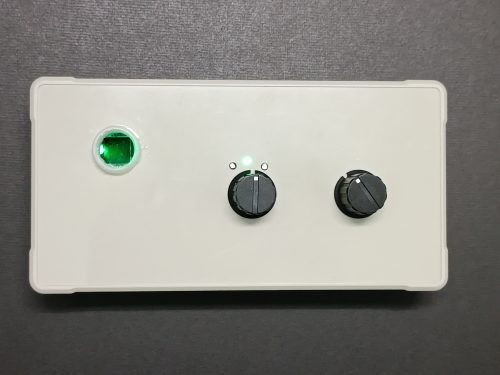
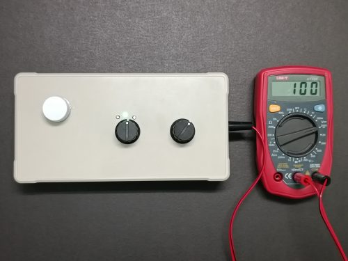
| (Fig. 169) Transmittance in near darkness | (Fig. 170) Colorimeter in operation |
b. Colorimeter circuit
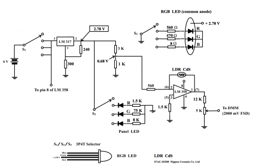
(Fig. 171) Colorimeter circuit
(C) Power supply
Power source of the circuit not only drive the Op-Amp LM 358, it also has to light up the tri-colour LED. The latter needs more current and 3V button-type lithium battery is not suitable for the job. Four AAA zinc-carbon cells connected in series providing a DC 6 V is a suitable power supply for the circuit. The power supply has to be regulated because circuit design requires a stable light source of irradiation. Adjustable voltage regulator IC LM 317 is selected because it suits the design purpose. Resistors 240 W and 300 W were used in the regulated circuit to provide a stable + 2.78 V as LEDs will burnt if supply voltage is over 3V. Regulated voltage is calculated as follows:
![]()
Because of value error of resistors, regulated voltage is measured to be 2.78 V instead of 2.81 V. LM 358 does not need regulated power supply as all Op-Amp linear ICs are designed to provide stable output within a range of acceptable supply voltage.
(D) Circuit description
(i) Selection of RGB LED wavelengths
A 3P4T selector is used (i) as an ON/OFF switch, (ii) to select red monochromatic light (mainly 625 nm), green monochromatic light (mainly 520 nm) and blue monochromatic light (mainly 470 nm).
(ii) Input to Op-Amp LM 358
One unit of dual Op-Amp LM 358 is connected as an inverting amplifier with pin 2 (the inverting input) receiving the source signal. Pin 2 of LM 317 when connected to a 3K and a 1K resistor in series will tap off [2.78 x (![]() )] V or 0.7 V. However, the resistor ladder circuit is in fact connected to the peripheral component network. The measured tapped p.d. is 0.68 V instead of the expected 0.7 V. This positive p.d. when input to the inverting amplifier has to do extra calculation to obtain the output p.d. in addition to the simple formula of Vout = Vin (
)] V or 0.7 V. However, the resistor ladder circuit is in fact connected to the peripheral component network. The measured tapped p.d. is 0.68 V instead of the expected 0.7 V. This positive p.d. when input to the inverting amplifier has to do extra calculation to obtain the output p.d. in addition to the simple formula of Vout = Vin ( ![]() ), see next paragraph.
), see next paragraph.
(iii) Voltage amplification and variation of light intensity
The central component of the circuit is the LDR CdS light sensitive resistor (Fig. 174). When irradiated by LED green light, its resistance is about 3.5 KΩ and when the light beam is blocked, the resistance will increase to about 45 KΩ. When this LDR is connected to pins 1 and 2, inverting amplification involving resistor 560 Ω results in magnifying factors of (i) normal light of (-3500/560)and (ii) near darkness of (- 45,000/560) or a range of ~ (- 6) to ~ (- 80). Revise Program (1) Topic 8.3.2 (b).
As the input to pin 2 of LM 358 is not a negative voltage i.e. + 0.68 V, output at pin 1 has to be calculated as follows:
Voltage calculation has to consider “ground”, i.e. actual 0V or the negative pole of the power source. However, the “ground” of an inverting amplifier is not 0V but the (-) terminal or pin 2 of LM 358. This position is called the “virtual ground”. As ideal behaviour requires the potential at the (-) and (+) terminal to be the same, pin 3, i.e. the (+) terminal, instead of connecting directly to the ground, has to be connected to a resistor to generate a p.d across the actual ground and the (+) terminal. This offset resistor is called the “bias resistor”. Value of this resistor is calculated as follows:
![]()
![]()
Upon irradiation by green light, the LDR CdS has a resistance about 3.5 KΩ and the p.d. developed across the 560 Ω resistor is 0.047 V. This input is amplified to about [(0.047) x (- 6)] V or – (~ 0.282) V. Thus, with reference to the equivalent circuit of Fig. 172, we have:
Output at pin 1 = 0.68 V+ 0.047 V + (~ – 0.282) V = ~ 0.445 V or ~ 445 mV
Range of output to DMM through the 5 K Ω variable resistor = 0 V to [(445) x (5/17)] mV = 0 to 131 mV
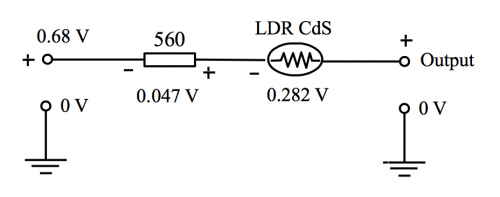
(Fig. 172) Inverting amplification p.d. equivalent circuit with polarity
In near darkness, the source signal was measured to be 0.738 V. The LDR CdS had an approximate resistance of 45 K W and the p.d. developed across the 560 Ω resistor is 0.0089 V. This input is amplified to ~ [(0.0089) x (- 80)] V or (~ – 0.712) V. Thus, the output voltage measured at pin 1, w.r.t. the ground of the 6V main voltage is [0.738 + (0.0089) + (~ – 0.712)] V = ~ 0.035 V, i.e. ~ 35 mV.
Range of output to DMM through the 5 K Ω variable resistor = 0 V to [(35) x (5/17)] mV = 0 to 10 mV. Thus, if a monochromatic green light source is irradiating a blank sample of cuvette containing deionized water, and by turning the 5 K W variable resistor knob, so that the DMM displays 100 mV, then the colorimeter is said to have been calibrated w.r.t. green light and the position of the 5 K W variable resistor knob is kept fixed.
(iv) Circuit performance
As voltage regulation by LM 317 provides source signal voltage and input p.d. is also stabilized, stability of the circuit depends largely on the quality of the LDR used. The design employs S7AC-03208 manufactured by Nippon Ceramic Co. Ltd which provides reliable sensitivity and stability. On the whole, circuit design possesses high display reproducibility and low drift. LM 358 is a single power supply Op-Amp IC, which requires only Vcc supply. Range of power voltage supply of LM 358 is 3V – 30V. Four AA zinc-carbon cells connected in series providing a 6V power source is suitable for the whole design, catering for both the IC and LEDs. Regulated voltage by LM 317 to provide 2.78 V for the LEDs, + 0.7 V for the IC input and raw 6 V for the Vcc of LM 358 is a decent way of power supply planning. The instrument is capable of continuous stable operation for a long period of time.
e. Construction details
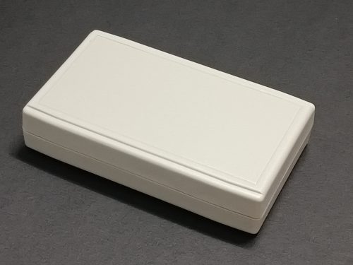
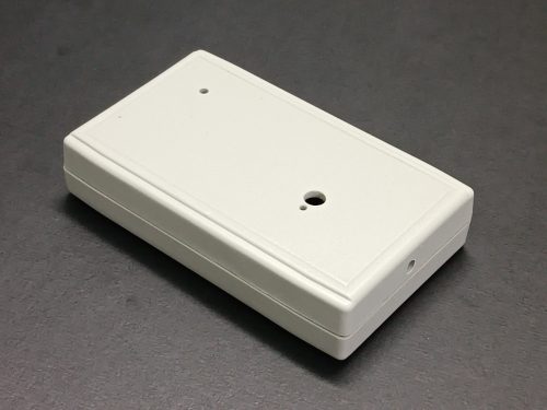
(i) Plastic utility box
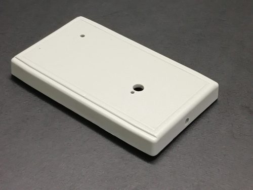
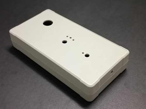
All parts of the instrument can be housed in a plastic utility box measuring (203 x 105 x 41) mm, including a bottom and a lid. Separate holes of different sizes are drilled on the lid to accommodate the (i) 3P4T selector, (ii) panel RGB LEDs, (iii) cuvette compartment, (iv) 5K W variable resistor and (v) output DC socket (Fig. 173).
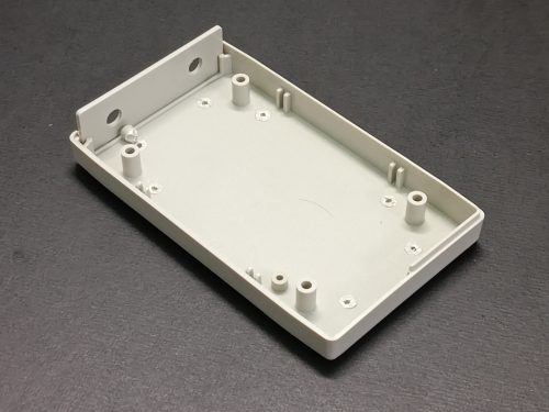
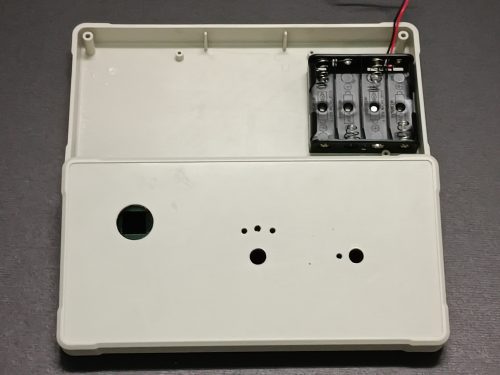
(ii) Power supply and battery holder
A battery holder which accommodates four 1.5VAA size zinc-carbon cells (6V) is firmly adhered to the bottom of the box by hot glue (Fig. 174).
|
|
|
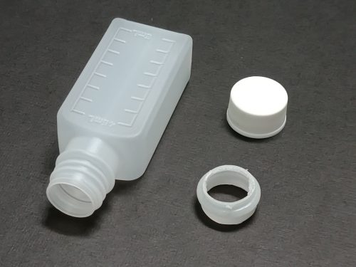
(Fig. 173) Utility box with various holes | (Fig. 174) Lid and bottom of the utility box with battery holder | (Fig. 175) Plastic medicine bottle, cap and top part |
(iii) Monochromatic light source
Unlike ten years ago, nowadays RGB tri-colour LED is becoming more and more popular. They are compact, inexpensive and can emit near monochromatic visible light. They emit strong red (625 nm), green (520 nm) and blue (470 nm) lights upon applying a DC voltage of < 3V. The method is superior than using RGB colour filters. Like all LEDs, these kind of RGB tri-colour LEDs are sensitive to supply voltage and will burn down when the supply voltage is over 3V DC.
(iv) Cuvette cavity and compartment
Select a plastic medicine bottle (60 cm3), the mouth of which can just accommodate a disposable cuvette with a dimension of (12.5 x 12.5 x 45) mm. Chop off the top part (Fig. 175), cement it to the large hole of the lid form a cuvette adapter. Fix it to the cavity hole with glue. Arrange and fix with trichloromethane four pieces of small strips of acrylate so that they form a shape of (井, Chinese meaning a well) (Fig. 176). Size of the central part of this strip combination should just allow a cuvette to pass through. Glue it to the bottom part of the cavity hole of the case cover (Fig. 177).
| (Fig. 173) Cuvette adapter and PVC strips combination | (Fig. 174) U-shaped acrylic stand with RGB LED and LDR CdS photoresistor | (Fig. 175) Cavity compartment allowing cuvette to go through |
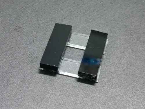
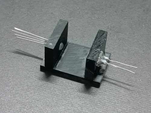
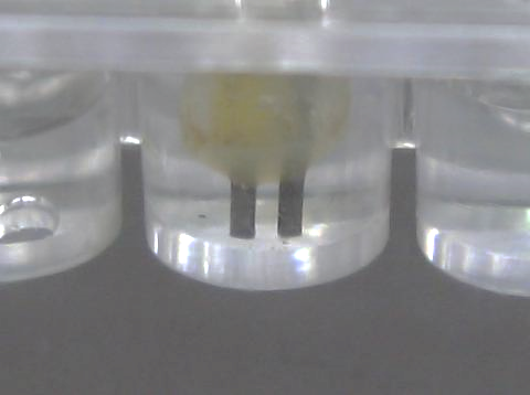
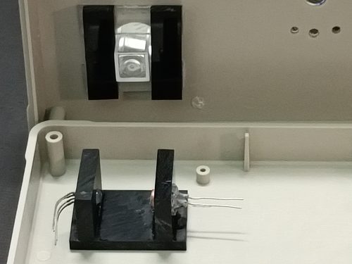
(v) Tri-colour LED light source and LDR stand
With the help of trichloromethane, cement 3 pieces of dark brown (or black, if available) thick acrylic sheets together to form a U-shaped stand. Drill opposite holes to hold the tri-colour LED and LDR respectively (Fig. 178). Fix them into position with hot glue or epoxy glue. Glue the whole assembly to the bottom part of the case to form a complete cuvette compartment (Fig. 179). There should be no room for movement once the cuvette has been inserted into the cavity, otherwise it may result in unstable DMM display.
(Fig. 179) Cavity compartment allowing cuvette to go through | (Fig. 180) Layout of universal PC board | (Fig. 181) Wired PC board, detached upper and lower parts of the plastic case |
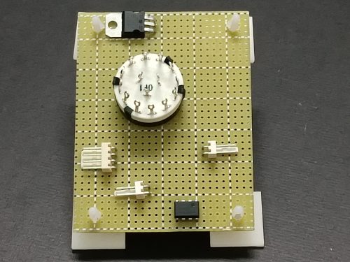
(vi) Component layout and circuit soldering
The whole circuit (Fig. 171) is soldered onto a universal PC board. Layout design should consider the need for easy maintenance (Fig. 180). As such, the completed PC board is made detachable and the upper and lower parts of the case can be separated (Fig. 181). Style of design is up to one’s favour, but convenience is the major factor to be considered.
Lastly, all parts liable to movement and hence loss of contact should be permanently sealed by hot glue. This includes soldered joints involving wires on the PC board and junctions of other wired-joints of components.
f. Preparation for experiment
(i) Calibration for a particular experiment
Calibration of the colorimeter has to be done with each experiment, as colour displayed by the chemical reaction varies.
Selection of monochromatic light source
Switch on the sensor and DMM, select the DC 2000 mV FS range and connect the sensor output to the DMM. Fill a clean cuvette (smooth opposite sides facing the light source and the LDR) with 3/4 full of deionized water. Place back the cuvette cap, select the red light source by turning the 3P4T selector and adjust the 5K variable resistor until a display of 100 mV is observed.
Remove the blank sample, fill the same clean cuvette 3/4 full with the colour sample. Observe the DMM reading, say 85 mV is displayed. Select the next light source, say the green light and again observe the DMM reading. Repeat the procedure for the blue light source. Determine the light source which give the lowest reading less than or equal to 85 mV. This is the chosen wavelength for the experiment. For a purple or brown solution, green light source should be used.
Set for full-scale calibration
Select the pre-determined light source suitable for the experiment. Place a clean cuvette filled with 3/4 full of deionized water. Adjust the 5K W variable resistor until a display of 100 mV is observed (Fig. 182). Remove the curvette, block the light path with an opaque object and observe the DMM reading for near darkness (Fig. 183).
(ii) Optical intensity measurement
After calibration, fix the position of the set full scale knob (5 KW variable resistor). Fill the clean cuvette 3/4 full with the sample solution and place back the cuvette. Wait till the display becomes steady and record the reading. If a value of 66 mV is observed, then the optical intensity of the solution can be interpreted as 66% transmittance w.r.t. the selected light source (Fig. 184).
(Fig. 182) Blank test | (Fig. 183) Test for complete darkness | (Fig. 184) 76% transmittance |
Expt (23): Determination of concentration of a sample of KMnO4 solution (page 163)
Expt (24): Determination of food dye present in a sample non-alcoholic drink (page 173)
Expt (25): Kinetic order of decolorization of phenolphthalein in a strongly alkaline solution (page 178)
Expt (26): Kinetuc order of the acidic oxidation of iodide ion by hydrogen peroxide (page 187)